Driverless AI: Credit Card Demo
This notebook provides an H2OAI Client workflow, of model building and scoring, that parallels the Driverless AI workflow.
Notes:
This is an early release of the Driverless AI Python client.
This notebook was tested in Driverless AI version 1.8.5.
Python 3.6 is the only supported version.
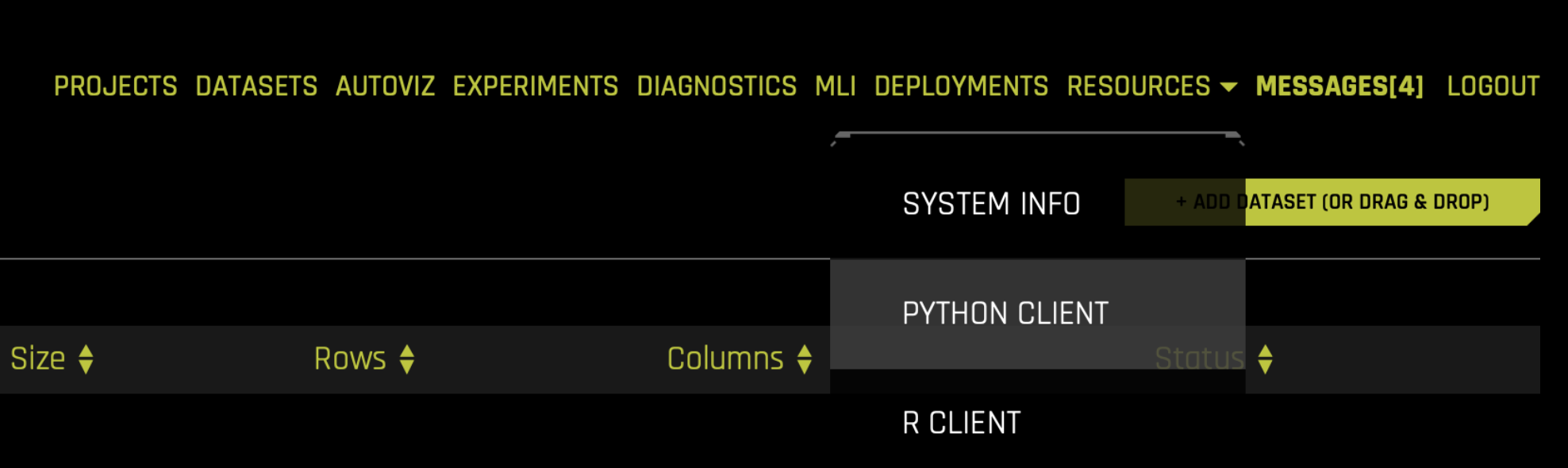
You must install the
h2oai_clientwheel to your local Python. This is available from the RESOURCES link in the top menu of the UI.
Workflow Steps
Build an Experiment with Python API:
Sign in
Import train & test set/new data
Specify experiment parameters
Launch Experiement
Examine Experiment
Download Predictions
Build an Experiment in Web UI and Access Through Python:
Get pointer to experiment
Score on New Data:
Score on new data with H2OAI model
Model Diagnostics on New Data:
Run model diagnostincs on new data with H2OAI model
Run Model Interpretation
Run model interpretation on the raw features
Run Model Interpretation on External Model Predictions
Build Scoring Pipelines
Build Python Scoring Pipeline
Build MOJO Scoring Pipeline
Build an Experiment with Python API
1. Sign In
Import the required modules and log in.
Pass in your credentials through the Client class which creates an authentication token to send to the Driverless AI Server. In plain English: to sign into the Driverless AI web page (which then sends requests to the Driverless Server), instantiate the Client class with your Driverless AI address and login credentials.
[1]:
from h2oai_client import Client
import matplotlib.pyplot as plt
import pandas as pd
[2]:
address = 'http://ip_where_driverless_is_running:12345'
username = 'username'
password = 'password'
h2oai = Client(address = address, username = username, password = password)
# make sure to use the same user name and password when signing in through the GUI

2. Upload Datasets
Upload training and testing datasets from the Driverless AI /data folder.
You can provide a training, validation, and testing dataset for an experiment. The validation and testing dataset are optional. In this example, we will provide only training and testing.
[3]:
train_path = '/data/Kaggle/CreditCard/CreditCard-train.csv'
test_path = '/data/Kaggle/CreditCard/CreditCard-test.csv'

train = h2oai.create_dataset_sync(train_path)
test = h2oai.create_dataset_sync(test_path)
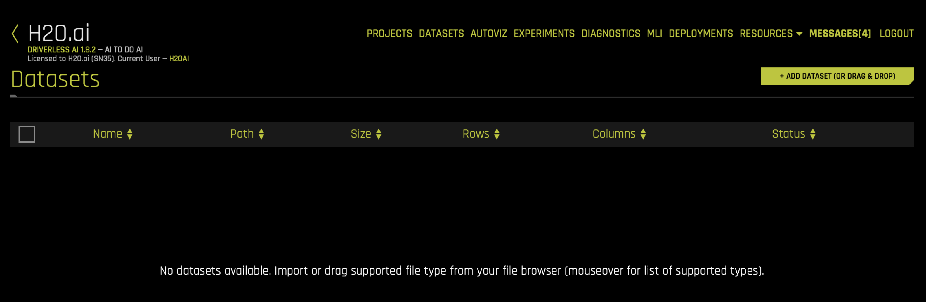
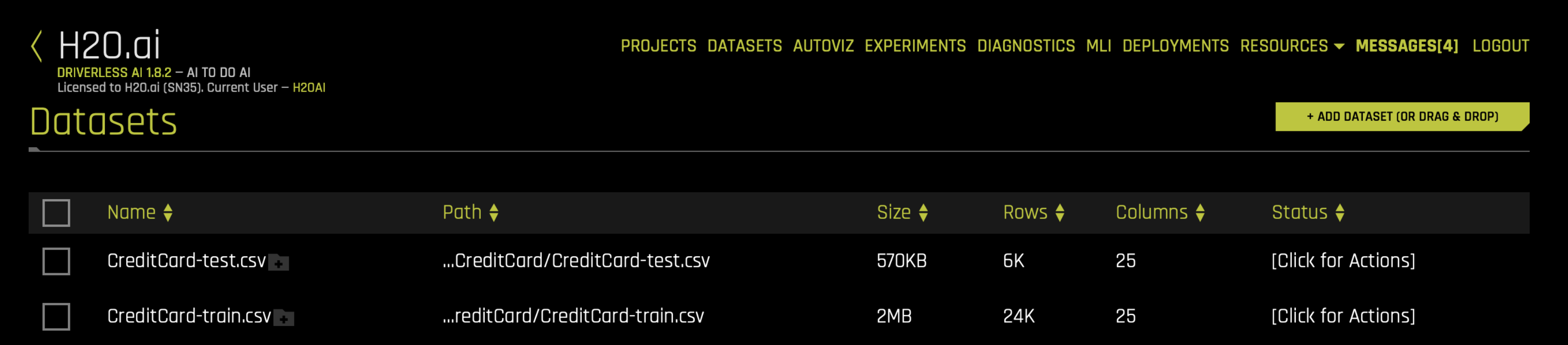
Equivalent Steps in Driverless: Uploading Train & Test CSV Files
3. Set Experiment Parameters
We will now set the parameters of our experiment. Some of the parameters include:
Target Column: The column we are trying to predict.
Dropped Columns: The columns we do not want to use as predictors such as ID columns, columns with data leakage, etc.
Weight Column: The column that indicates the per row observation weights. If
None, each row will have an observation weight of 1.Fold Column: The column that indicates the fold. If
None, the folds will be determined by Driverless AI.Is Time Series: Whether or not the experiment is a time-series use case.
For information on the experiment settings, refer to the Experiment Settings.
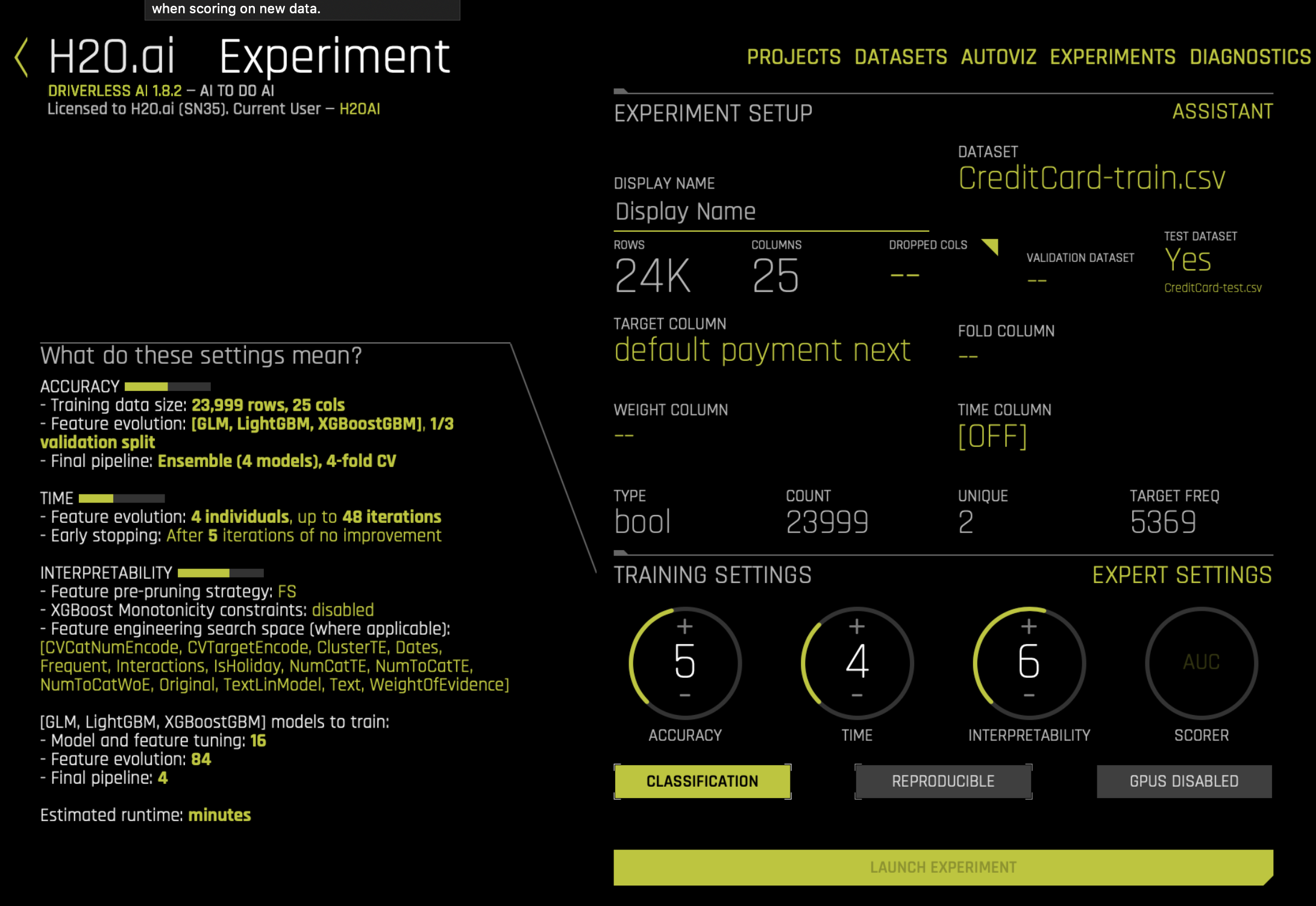
For this example, we will be predicting ``default payment next month``. The parameters that control the experiment process are: accuracy, time, and interpretability. We can use the get_experiment_preview_sync function to get a sense of what will happen during the experiment.
We will start out by seeing what the experiment will look like with accuracy, time, and interpretability all set to 5.
[4]:
target="default payment next month"
exp_preview = h2oai.get_experiment_preview_sync(dataset_key= train.key
                                                , validset_key=''
                                                , classification=True
                                                , dropped_cols=[]
                                                , target_col=target
                                                , is_time_series=False
                                                , enable_gpus=False
                                                , accuracy=5, time=5, interpretability=5
                                                , reproducible=True
                                                , resumed_experiment_id=''
                                                , time_col=''
                                                , config_overrides=None)
exp_preview
[4]:
['ACCURACY [5/10]:',
 '- Training data size: *23,999 rows, 25 cols*',
 '- Feature evolution: *[LightGBM, XGBoostGBM]*, *1/3 validation split*',
 '- Final pipeline: *Ensemble (4 models), 4-fold CV*',
 '',
 'TIME [5/10]:',
 '- Feature evolution: *4 individuals*, up to *66 iterations*',
 '- Early stopping: After *10* iterations of no improvement',
 '',
 'INTERPRETABILITY [5/10]:',
 '- Feature pre-pruning strategy: None',
 '- Monotonicity constraints: disabled',
 '- Feature engineering search space: [CVCatNumEncode, CVTargetEncode, ClusterDist, ClusterTE, Frequent, Interactions, NumCatTE, NumToCatTE, NumToCatWoE, Original, TruncSVDNum, WeightOfEvidence]',
 '',
 '[LightGBM, XGBoostGBM] models to train:',
 '- Model and feature tuning: *16*',
 '- Feature evolution: *104*',
 '- Final pipeline: *4*',
 '',
 'Estimated runtime: *minutes*',
 'Auto-click Finish/Abort if not done in: *1 day*/*7 days*']
With these settings, the Driverless AI experiment will train about 124 models: * 16 for model and feature tuning * 104 for feature evolution * 4 for the final pipeline
When we start the experiment, we can either:
specify parameters
use Driverless AI to suggest parameters
Driverless AI can suggest the parameters based on the dataset and target column. Below we will use the ``get_experiment_tuning_suggestion`` to see what settings Driverless AI suggests.
[5]:
# let Driverless suggest parameters for experiment
params = h2oai.get_experiment_tuning_suggestion(dataset_key = train.key, target_col = target,
                                                is_classification = True, is_time_series = False,
                                                config_overrides = None, cols_to_drop=[])

params.dump()
[5]:
{'dataset': {'key': '6f09ae32-33dc-11ea-ba27-0242ac110002',
  'display_name': ''},
 'resumed_model': {'key': '', 'display_name': ''},
 'target_col': 'default payment next month',
 'weight_col': '',
 'fold_col': '',
 'orig_time_col': '',
 'time_col': '',
 'is_classification': True,
 'cols_to_drop': [],
 'validset': {'key': '', 'display_name': ''},
 'testset': {'key': '', 'display_name': ''},
 'enable_gpus': True,
 'seed': False,
 'accuracy': 5,
 'time': 4,
 'interpretability': 6,
 'score_f_name': 'AUC',
 'time_groups_columns': [],
 'unavailable_columns_at_prediction_time': [],
 'time_period_in_seconds': None,
 'num_prediction_periods': None,
 'num_gap_periods': None,
 'is_timeseries': False,
 'config_overrides': None}
Driverless AI has found that the best parameters are to set ``accuracy = 5``, ``time = 4``, ``interpretability = 6``. It has selected ``AUC`` as the scorer (this is the default scorer for binomial problems).
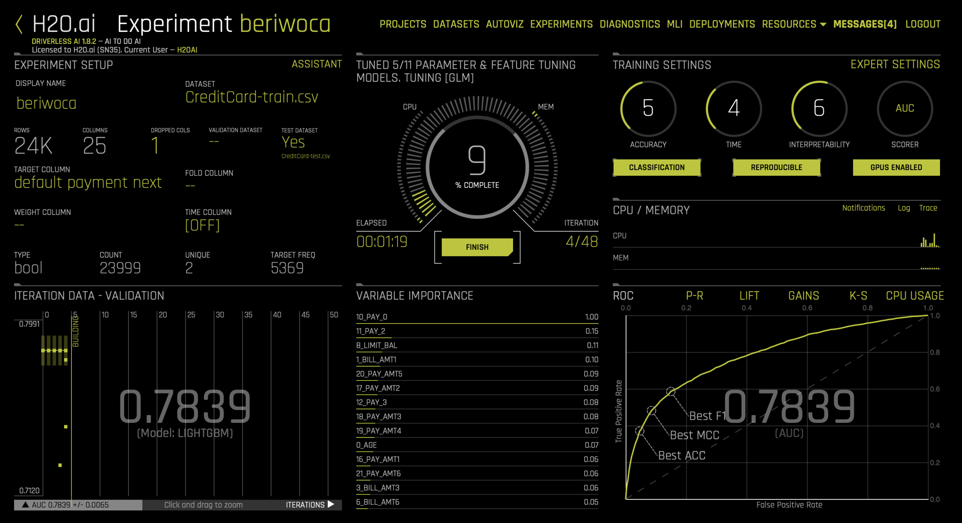
Equivalent Steps in Driverless: Set the Knobs, Configuration & Launch
4. Launch Experiment: Feature Engineering + Final Model Training
Launch the experiment using the parameters that Driverless AI suggested along with the testset, scorer, and seed that were added. We can launch the experiment with the suggested parameters or create our own.
[6]:
experiment = h2oai.start_experiment_sync(dataset_key=train.key,
                                         testset_key = test.key,
                                         target_col=target,
                                         is_classification=True,
                                         accuracy=5,
                                         time=4,
                                         interpretability=6,
                                         scorer="AUC",
                                         enable_gpus=True,
                                         seed=1234,
                                         cols_to_drop=['ID'])
5. Examine Experiment
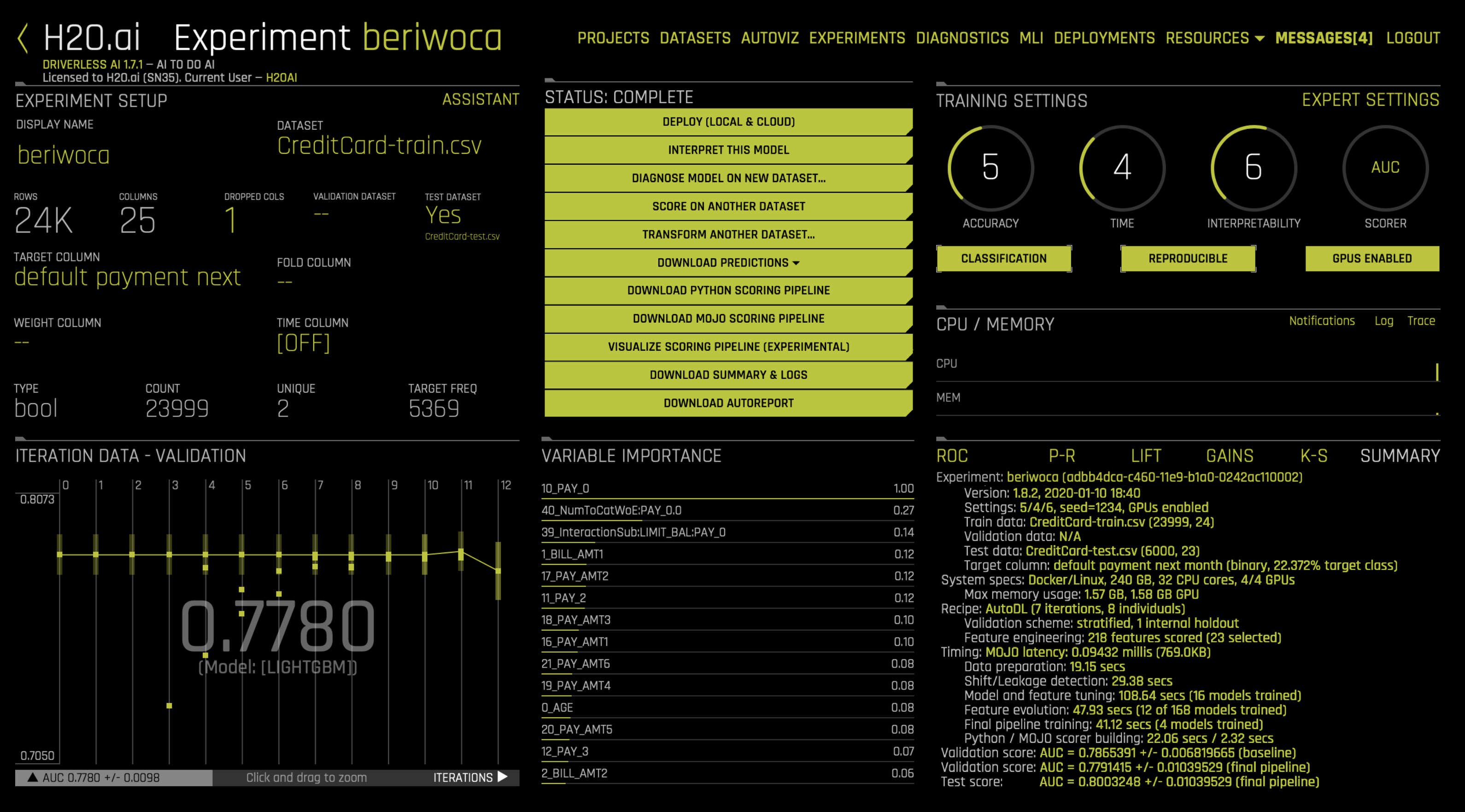
View the final model score for the validation and test datasets. When feature engineering is complete, an ensemble model can be built depending on the accuracy setting. The experiment object also contains the score on the validation and test data for this ensemble model. In this case, the validation score is the score on the training cross-validation predictions.
[7]:
print("Final Model Score on Validation Data: " + str(round(experiment.valid_score, 3)))
print("Final Model Score on Test Data: " + str(round(experiment.test_score, 3)))
Final Model Score on Validation Data: 0.779
Final Model Score on Test Data: 0.8
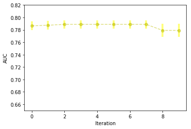
The experiment object also contains the scores calculated for each iteration on bootstrapped samples on the validation data. In the iteration graph in the UI, we can see the mean performance for the best model (yellow dot) and +/- 1 standard deviation of the best model performance (yellow bar).
This information is saved in the experiment object.
[8]:
# Add scores from experiment iterations
iteration_data = h2oai.list_model_iteration_data(experiment.key, 0, len(experiment.iteration_data))
iterations = list(map(lambda iteration: iteration.iteration, iteration_data))
scores_mean = list(map(lambda iteration: iteration.score_mean, iteration_data))
scores_sd = list(map(lambda iteration: iteration.score_sd, iteration_data))

# Add score from final ensemble
iterations = iterations + [max(iterations) + 1]
scores_mean = scores_mean + [experiment.valid_score]
scores_sd = scores_sd + [experiment.valid_score_sd]

plt.figure()
plt.errorbar(iterations, scores_mean, yerr=scores_sd, color = "y",
             ecolor='yellow', fmt = '--o', elinewidth = 4, alpha = 0.5)
plt.xlabel("Iteration")
plt.ylabel("AUC")
plt.ylim([0.65, 0.82])
plt.show();
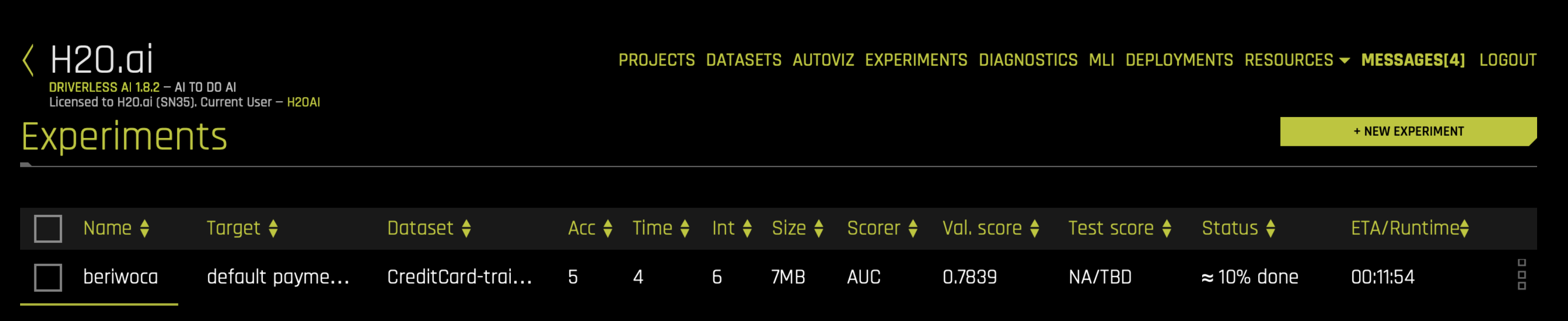
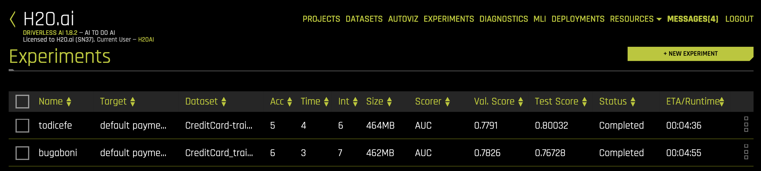
Equivalent Steps in Driverless: View Results
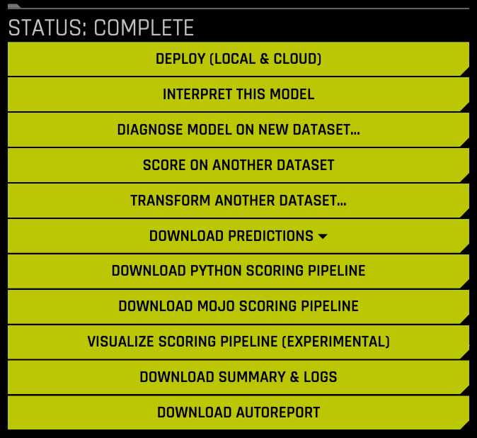
6. Download Results
Once an experiment is complete, we can see that the UI presents us options of downloading the:
predictions
on the (holdout) train data
on the test data
experiment summary - summary of the experiment including feature importance
We will show an example of downloading the test predictions below. Note that equivalent commands can also be run for downloading the train (holdout) predictions.
[9]:
h2oai.download(src_path=experiment.test_predictions_path, dest_dir=".")
[9]:
'./test_preds.csv'
[10]:
test_preds = pd.read_csv("./test_preds.csv")
test_preds.head()
[10]:
| default payment next month.0 | default payment next month.1 | |
|---|---|---|
| 0 | 0.399347 | 0.600653 |
| 1 | 0.858302 | 0.141698 |
| 2 | 0.938646 | 0.061354 |
| 3 | 0.619994 | 0.380006 |
| 4 | 0.865251 | 0.134749 |
Build an Experiment in Web UI and Access Through Python
It is also possible to use the Python API to examine an experiment that was started through the Web UI using the experiment key.
1. Get pointer to experiment
You can get a pointer to the experiment by referencing the experiment key in the Web UI.
[11]:
# Get list of experiments
experiment_list = list(map(lambda x: x.key, h2oai.list_models(offset=0, limit=100).models))
experiment_list
[11]:
['7f7b429e-33dc-11ea-ba27-0242ac110002',
 '0be7d94a-33d8-11ea-ba27-0242ac110002',
 '2e6bbcfa-30a1-11ea-83f9-0242ac110002',
 '3c06c58c-27fd-11ea-9e09-0242ac110002',
 'a3c6dfda-2353-11ea-9f4a-0242ac110002',
 '15fe0c0a-203d-11ea-97b6-0242ac110002']
[12]:
# Get pointer to experiment
experiment = h2oai.get_model_job(experiment_list[0]).entity
Score on New Data
You can use the Python API to score on new data. This is equivalent to the SCORE ON ANOTHER DATASET button in the Web UI. The example below scores on the test data and then downloads the predictions.
Pass in any dataset that has the same columns as the original training set. If you passed a test set during the H2OAI model building step, the predictions already exist.
1. Score Using the H2OAI Model
The following shows the predicted probability of default for each record in the test.
[13]:
prediction = h2oai.make_prediction_sync(experiment.key, test.key, output_margin = False, pred_contribs = False)
pred_path = h2oai.download(prediction.predictions_csv_path, '.')
pred_table = pd.read_csv(pred_path)
pred_table.head()
[13]:
| default payment next month.0 | default payment next month.1 | |
|---|---|---|
| 0 | 0.399347 | 0.600653 |
| 1 | 0.858302 | 0.141698 |
| 2 | 0.938646 | 0.061354 |
| 3 | 0.619994 | 0.380006 |
| 4 | 0.865251 | 0.134749 |
We can also get the contribution each feature had to the final prediction by setting pred_contribs = True. This will give us an idea of how each feature effects the predictions.
[14]:
prediction_contributions = h2oai.make_prediction_sync(experiment.key, test.key,
                                                      output_margin = False, pred_contribs = True)
pred_contributions_path = h2oai.download(prediction_contributions.predictions_csv_path, '.')
pred_contributions_table = pd.read_csv(pred_contributions_path)
pred_contributions_table.head()
[14]:
| contrib_0_AGE | contrib_10_PAY_0 | contrib_11_PAY_2 | contrib_12_PAY_3 | contrib_13_PAY_4 | contrib_14_PAY_5 | contrib_15_PAY_6 | contrib_16_PAY_AMT1 | contrib_17_PAY_AMT2 | contrib_18_PAY_AMT3 | ... | contrib_22_SEX | contrib_2_BILL_AMT2 | contrib_3_BILL_AMT3 | contrib_4_BILL_AMT4 | contrib_5_BILL_AMT5 | contrib_6_BILL_AMT6 | contrib_7_EDUCATION | contrib_8_LIMIT_BAL | contrib_9_MARRIAGE | contrib_bias | |
|---|---|---|---|---|---|---|---|---|---|---|---|---|---|---|---|---|---|---|---|---|---|
| 0 | -0.017284 | 1.559683 | 0.336257 | -0.004992 | -0.009970 | -0.028749 | -0.046268 | 0.064267 | -0.021834 | -0.015015 | ... | 0.000940 | -0.039787 | -0.010946 | -0.034707 | 0.025392 | 0.013222 | 0.008324 | 0.163888 | -0.046693 | -1.507163 |
| 1 | -0.006587 | -0.283259 | -0.058643 | -0.014668 | -0.025089 | -0.021999 | -0.021543 | 0.091787 | -0.061340 | -0.057014 | ... | 0.056241 | -0.041630 | 0.027173 | -0.000515 | -0.017727 | -0.006212 | 0.029378 | 0.323900 | -0.066966 | -1.507163 |
| 2 | -0.017300 | -0.347706 | -0.061856 | -0.027669 | -0.018144 | -0.011283 | -0.017874 | 0.047035 | -0.229566 | -0.065025 | ... | 0.024883 | -0.041808 | -0.024132 | -0.050757 | -0.016839 | -0.021221 | 0.020798 | -0.335934 | -0.069577 | -1.507163 |
| 3 | -0.064728 | 0.916047 | 0.081330 | 0.153046 | 0.166219 | 0.170304 | 0.077901 | 0.059009 | 0.052934 | 0.125983 | ... | -0.001882 | 0.050526 | 0.059255 | -0.033044 | -0.001438 | 0.011796 | -0.858484 | 0.100657 | -0.043778 | -1.507163 |
| 4 | -0.029481 | -0.260402 | -0.058225 | -0.155098 | -0.047545 | -0.022028 | -0.024870 | 0.076568 | 0.119231 | 0.123152 | ... | 0.021810 | -0.015791 | -0.161386 | -0.032228 | -0.005339 | -0.016350 | 0.010969 | 0.112077 | -0.039533 | -1.507163 |
5 rows × 24 columns
We will examine the contributions for our first record more closely.
[15]:
contrib = pd.DataFrame(pred_contributions_table.iloc[0][1:])
contrib.columns = ["contribution"]
contrib["abs_contribution"] = contrib.contribution.abs()
contrib.sort_values(by="abs_contribution", ascending=False)[["contribution"]].head()
[15]:
| contribution | |
|---|---|
| contrib_10_PAY_0 | 1.559683 |
| contrib_bias | -1.507163 |
| contrib_11_PAY_2 | 0.336257 |
| contrib_8_LIMIT_BAL | 0.163888 |
| contrib_1_BILL_AMT1 | -0.100378 |
The clusters from this customer’s: PAY_0, PAY_2, and LIMIT_BAL had the greatest impact on their prediction. Since the contribution is positive, we know that it increases the probability that they will default.
Model Diagnostics on New Data
You can use the Python API to also perform model diagnostics on new data. This is equivalent to the Model Diagnostics tab in the Web UI.
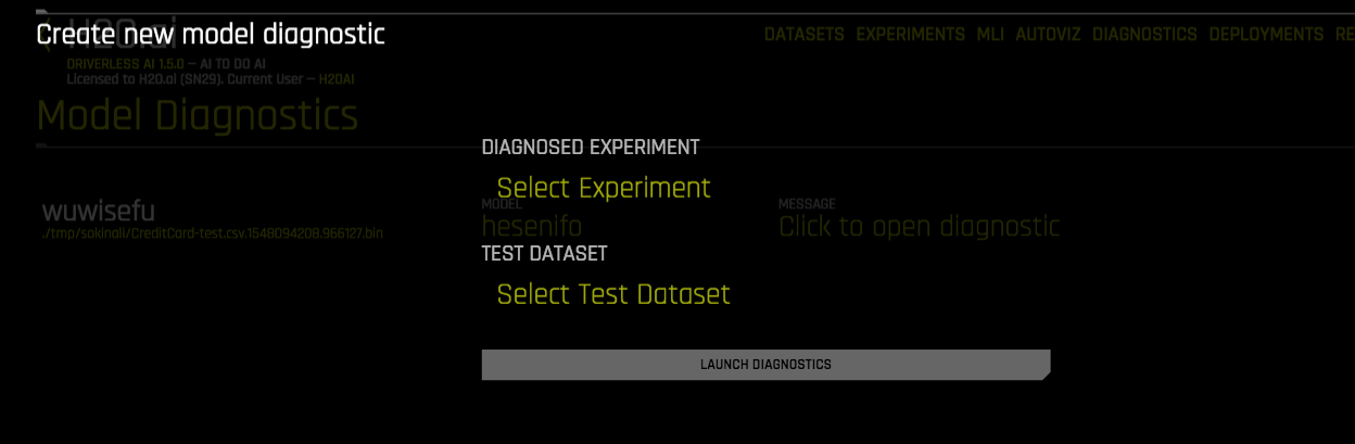
1. Run model diagnostincs on new data with H2OAI model
The example below performs model diagnostics on the test dataset but any data with the same columns can be selected.
[16]:
test_diagnostics = h2oai.make_model_diagnostic_sync(experiment.key, test.key)
[17]:
[{'scorer': x.score_f_name, 'score': x.score} for x in test_diagnostics.scores]
[17]:
[{'scorer': 'ACCURACY', 'score': 0.8326666666666667},
 {'scorer': 'AUC', 'score': 0.8003248324279806},
 {'scorer': 'AUCPR', 'score': 0.5805185237503238},
 {'scorer': 'F05', 'score': 0.5957993999142734},
 {'scorer': 'F1', 'score': 0.5563139931740614},
 {'scorer': 'F2', 'score': 0.6467051171922935},
 {'scorer': 'GINI', 'score': 0.6006496648559612},
 {'scorer': 'LOGLOSS', 'score': 0.406033500339215},
 {'scorer': 'MACROAUC', 'score': 0.8003248324279806},
 {'scorer': 'MCC', 'score': 0.4517110838237804}]
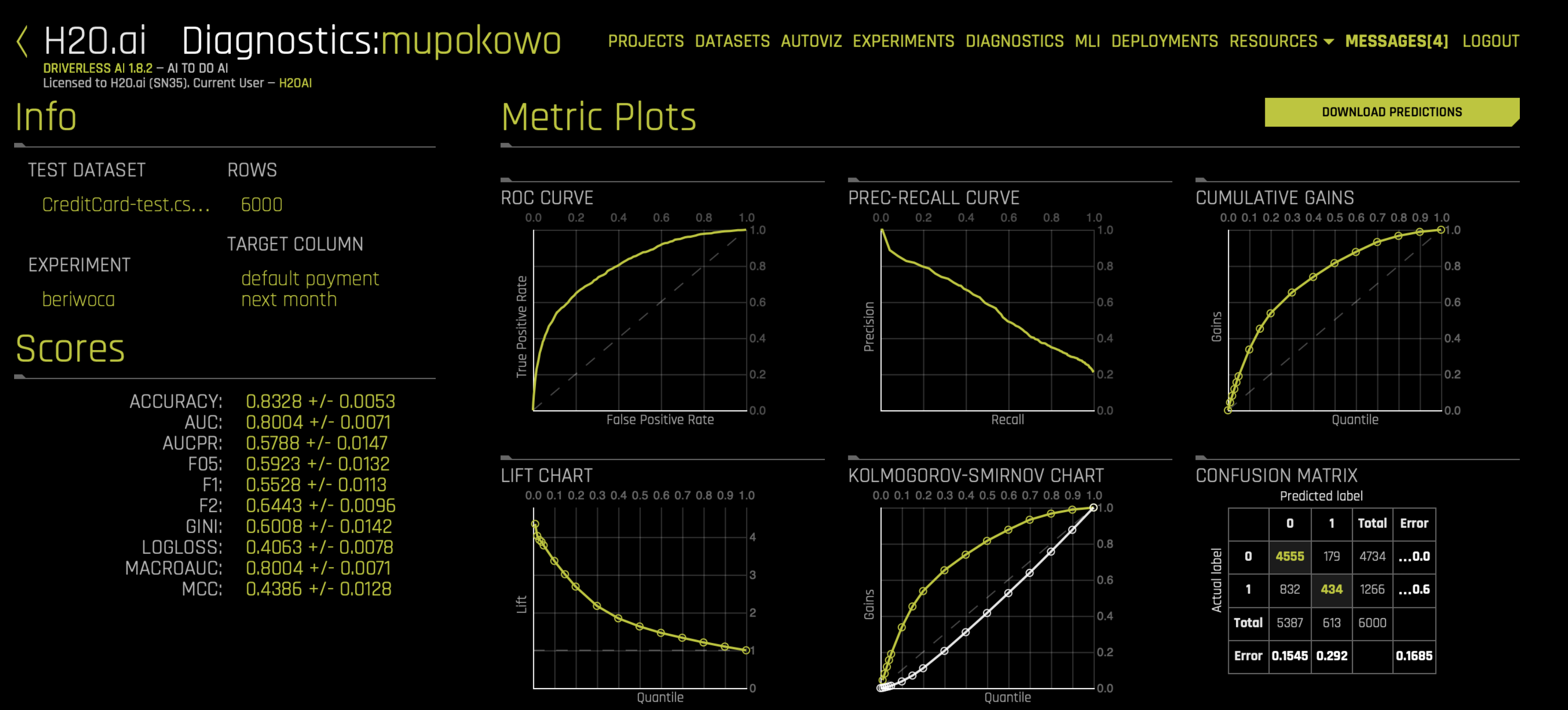
Here is the same model diagnostics displayed in the UI:
Run Model Interpretation
Once we have completed an experiment, we can interpret our H2OAI model. Model Interpretability is used to provide model transparency and explanations. More information on Model Interpretability can be found here: http://docs.h2o.ai/driverless-ai/latest-stable/docs/userguide/interpreting.html.
1. Run Model Interpretation on the Raw Data
We can run the model interpretation in the Python client as shown below. By setting the parameter, use_raw_features to True, we are interpreting the model using only the raw features in the data. This will not use the engineered features we saw in our final model’s features to explain the data.
[18]:
mli_experiment = h2oai.run_interpretation_sync(dai_model_key = experiment.key,
                                               dataset_key = train.key,
                                               target_col = target,
                                               use_raw_features = True)
This is equivalent to clicking Interpet this Model on Original Features in the UI once the experiment has completed.
Once our interpretation is finished, we can navigate to the MLI tab in the UI to see our interpreted model.
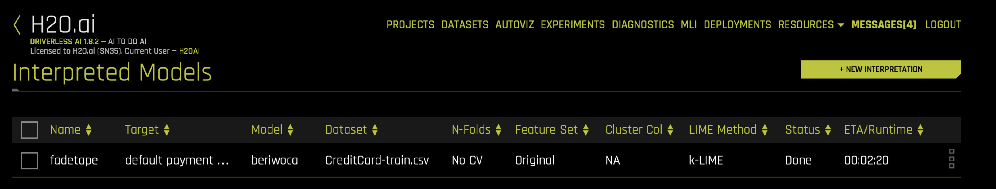
We can also see the list of interpretations using the Python Client:
[19]:
# Get list of interpretations
mli_list = list(map(lambda x: x.key, h2oai.list_interpretations(offset=0, limit=100)))
mli_list
[19]:
['2ff44e94-33de-11ea-ba27-0242ac110002',
 '6ce9e9f6-33db-11ea-ba27-0242ac110002']
2. Run Model Interpretation on External Model Predictions
Model Interpretation does not need to be run on a Driverless AI experiment. We can also train an external model and run Model Interpretability on the predictions. In this next section, we will walk through the steps to interpret an external model.
Train External Model
We will begin by training a model with scikit-learn. Our end goal is to use Driverless AI to interpret the predictions made by our scikit-learn model.
[25]:
# Dataset must be located where Python client is running - you may need to download it locally
train_pd = pd.read_csv(train_path)
[26]:
from sklearn.ensemble import GradientBoostingClassifier

predictors = list(set(train_pd.columns) - set([target]))

gbm_model = GradientBoostingClassifier(random_state=10)
gbm_model.fit(train_pd[predictors], train_pd[target])
[26]:
GradientBoostingClassifier(criterion='friedman_mse', init=None,
                           learning_rate=0.1, loss='deviance', max_depth=3,
                           max_features=None, max_leaf_nodes=None,
                           min_impurity_decrease=0.0, min_impurity_split=None,
                           min_samples_leaf=1, min_samples_split=2,
                           min_weight_fraction_leaf=0.0, n_estimators=100,
                           n_iter_no_change=None, presort='auto',
                           random_state=10, subsample=1.0, tol=0.0001,
                           validation_fraction=0.1, verbose=0,
                           warm_start=False)
[27]:
predictions = gbm_model.predict_proba(train_pd[predictors])
predictions[0:5]
[27]:
array([[0.20060823, 0.79939177],
       [0.57311744, 0.42688256],
       [0.88034896, 0.11965104],
       [0.86483594, 0.13516406],
       [0.87349721, 0.12650279]])
Interpret on External Predictions
Now that we have the predictions from our scikit-learn GBM model, we can call Driverless AI’s ``h2o_ai.run_interpretation_sync`` to create the interpretation screen.
[28]:
train_gbm_path = "./CreditCard-train-gbm_pred.csv"
predictions = pd.concat([train_pd, pd.DataFrame(predictions[:, 1], columns = ["p1"])], axis = 1)
predictions.to_csv(path_or_buf=train_gbm_path, index = False)
[29]:
train_gbm_pred = h2oai.upload_dataset_sync(train_gbm_path)
[30]:
mli_external = h2oai.run_interpretation_sync(dai_model_key = "", # no experiment key
                                             dataset_key = train_gbm_pred.key,
                                             target_col = target,
                                             prediction_col = "p1")
We can also run Model Interpretability on an external model in the UI as shown below:
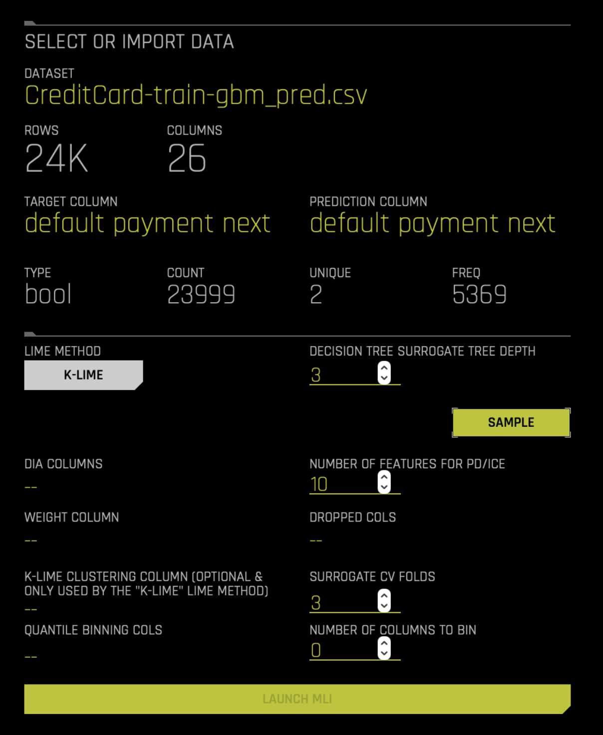
[31]:
# Get list of interpretations
mli_list = list(map(lambda x: x.key, h2oai.list_interpretations(offset=0, limit=100)))
mli_list
[31]:
['minemutu', 'nutiduha', 'senikahi']
Build Scoring Pipelines
In our last section, we will build the scoring pipelines from our experiment. There are two scoring pipeline options:
Python Scoring Pipeline: requires Python runtime
MOJO Scoring Pipeline: requires Java runtime
Documentation on the scoring pipelines is provided here: http://docs.h2o.ai/driverless-ai/latest-stable/docs/userguide/python-mojo-pipelines.html.
The experiment screen shows two scoring pipeline buttons: Download Python Scoring Pipeline or Build MOJO Scoring Pipeline. Driverless AI determines if any scoring pipeline should be automatically built based on the config.toml file. In this example, we have run Driverless AI with the settings:
# Whether to create the Python scoring pipeline at the end of each experiment
make_python_scoring_pipeline = true

# Whether to create the MOJO scoring pipeline at the end of each experiment
# Note: Not all transformers or main models are available for MOJO (e.g. no gblinear main model)
make_mojo_scoring_pipeline = false
Therefore, only the Python Scoring Pipeline will be built by default.
1. Build Python Scoring Pipeline
The Python Scoring Pipeline has been built by default based on our config.toml settings. We can get the path to the Python Scoring Pipeline in our experiment object.
[32]:
experiment.scoring_pipeline_path
[32]:
'h2oai_experiment_daguwofe/scoring_pipeline/scorer.zip'
We can also build the Python Scoring Pipeline - this is useful if the ``make_python_scoring_pipeline`` option was set to false.
[58]:
python_scoring_pipeline = h2oai.build_scoring_pipeline_sync(experiment.key)
[59]:
python_scoring_pipeline.file_path
[59]:
'h2oai_experiment_adbb4dca-c460-11e9-b1a0-0242ac110002/scoring_pipeline/scorer.zip'
Now we will download the scoring pipeline zip file.
[60]:
h2oai.download(python_scoring_pipeline.file_path, dest_dir=".")
[60]:
'./scorer.zip'
2. Build MOJO Scoring Pipeline
The MOJO Scoring Pipeline has not been built by default because of our config.toml settings. We can build the MOJO Scoring Pipeline using the Python client. This is equivalent to selecting the Build MOJO Scoring Pipeline on the experiment screen.
[61]:
mojo_scoring_pipeline = h2oai.build_mojo_pipeline_sync(experiment.key)
[62]:
mojo_scoring_pipeline.file_path
[62]:
'h2oai_experiment_adbb4dca-c460-11e9-b1a0-0242ac110002/mojo_pipeline/mojo.zip'
Now we can download the scoring pipeline zip file.
[63]:
h2oai.download(mojo_scoring_pipeline.file_path, dest_dir=".")
[63]:
'./mojo.zip'
Once the MOJO Scoring Pipeline is built, the Build MOJO Scoring Pipeline changes to Download MOJO Scoring Pipeline.
[ ]: